Hello friends again! I'm currently working on a Face Recognition project, using average half faces. I'm using the eigenface technique for face recognition. Since I'm a novice myself in this area, I did an extensive search on the net for understanding the bare concepts of this technique. So here I'm posting all the knowledge I gathered. I hope it helps you in thinking in the right direction if you are confused.

Please note that I have collected this information from many sources, so at the end of my post I'm providing the references. Heartfelt thanks to all of them. And by mistake, if I published someone's work here and did not mention his/her name, kindly inform me through mail, along with a link to your work, and I will be glad to correct my mistake.

Also, at some places I have pasted images of some symbols instead of inserting them, (like using instead of writing Φ_i ) because I haven't yet got the hang of font and formatting in this blog. So forgive me for that. 

So here we go!

Face Recognition using Eigenfaces, with an introduction to using the Average Half Face

Introduction

In today's networked world, the need to maintain the security of information or physical property is becoming both increasingly important and increasingly difficult. From time to time we hear about the crimes of credit card fraud, computer break-ins by hackers, or security breaches in a company or government building. In most of these crimes, the criminals were taking advantage of a fundamental flaw in the conventional access control systems: the systems do not grant access by "who we are", but by "what we have", such as ID cards, keys, passwords, PIN numbers, or mother's maiden name. None of these means are really define us. Rather, they merely are means to authenticate us. It goes without saying that if someone steals, duplicates, or acquires these identity means, he or she will be able to access our data or our personal property any time they want. Recently, technology became available to allow verification of "true" individual identity. This technology is based in a field called "biometrics". Biometric access control are automated methods of verifying or recognizing the identity of a living person on the basis of some physiological characteristics, such as fingerprints or facial features, or some aspects of the person's behavior, like his/her handwriting style or keystroke patterns. Since biometric systems identify a person by biological characteristics, they are difficult to forge.

Face recognition is one of the few biometric methods that possess the merits of both high accuracy and low intrusiveness. It has the accuracy of a physiological approach without being intrusive. For this reason, since the early 70's, face recognition has drawn the attention of researchers in fields from security, psychology, and image processing, to computer vision. While network security and access control are it most widely discussed applications, face recognition has also proven useful in other multimedia information processing areas. It could also be used to obtain quick access to medical, criminal, or any type of records. Solving this problem is important because it could allow personnel to take preventive action, provide better service - in the case of a doctor’s appointment, or allow a person access to a secure area.

Many face recognition algorithms have been developed and each has its strengths. Each share a common element which is that they all input a full face image into the algorithm. However, none of the methods currently exploit the inherent symmetry of the face for recognition. In this paper we demonstrate the effectiveness of using the average-half-face as an input to face recognition algorithms for an increase in accuracy and potential decrease in storage and computation time. The average half-face is a transformation method that attempts to preserve the bilateral symmetry that is present in the face. We will implement this technique using an approach called Eigenfaces. Eigenfaces, based on principal components analysis (PCA), is arguably the best known face recognition method and is used extensively as a benchmark for other methods.

Facial recognition was the source of motivation behind the creation of eigenfaces. For this use, eigenfaces have advantages over other techniques available, such as the system's speed and efficiency. Using eigenfaces is very fast, and able to functionally operate on lots of faces in very little time. Unfortunately, this type of facial recognition does have a drawback to consider: trouble recognizing faces when they are viewed with different levels of light or angles. For the system to work well, the faces need to be seen from a frontal view under similar lighting. Face recognition using eigenfaces has been shown to be quite accurate. By experimenting with the system to test it under variations of certain conditions, the following correct recognitions were found: an average of 96% with light variation, 85% with orientation variation, and 64% with size variation.

Generic Framework

In most cases, a face recognition algorithm can be divided into the following functional modules: a face image detector finds the locations of human faces from a normal picture against simple or complex background, and a face recognizer determines who this person is. Both the face detector and the face recognizer follow the same framework; they both have a feature extractor that transforms the pixels of the facial image into a useful vector representation, and a pattern recognizer that searches the database to find the best match to the incoming face image. The difference between the two is the following; in the face detection scenario, the pattern recognizer categorizes he incoming feature vector to one of the two image classes: “face” images and “non-face images. In the face recognition scenario, on the other hand, the recognizer classifies the feature vector (assuming it is from a “face” image) as “Smith’s face”, “Jane’s face”, or some other person’s face that is already registered in the database. The figure below depicts one example of the face recognition system.

Notice that there is an additional “eye localizer” in this system. Due to all kinds of the variations that may occur in the image (as discussed below), the face detector usually produces only an “approximate” location of the face. In order to find the “exact” location of the face for recognition, face recognition system designers often use the locations of both eyes for assistance. In this system, all the three functional modules (face detector, eye localizer, and face recognizer) follow the “feature extractor + pattern recognizer” schematics.

An Overview of the Eigenface method

Our aim is to represent a face as a linear combination of a set of eigen images. This set of eigenfaces (or eigenvectors) can be generated by performing a mathematical process called principal component analysis (PCA) on a large set of training images depicting different human faces. Thereafter, any human face can be considered to be a combination of this set of eigen faces.  For example, one's face might be composed of the average face plus 10% from eigenface 1, 55% from eigenface 2, and even -3% from eigenface 3.

Mathematically:

where   represents the   face with the mean subtracted from it,  represent weights and   the eigenvectors. 

The big idea is that you want to find a set of images (called Eigenfaces, which are nothing but Eigenvectors of the training data) that if you weigh and add together should give you back an image that you are interested in. The way you weight these basis images (i.e. the weight vector) could be used as a sort of a code for that image-of-interest and could be used as features for recognition. Remarkably, it does not take many eigenfaces combined together to achieve a fair approximation of most faces.

This can be represented aptly in a figure as:

In the above figure, a face that was in the training database was reconstructed by taking a weighted summation of all the basis faces (eigen faces) and then adding to them the mean face.

First of all the idea of Eigenfaces considers face recognition as a 2-D recognition problem; this is based on the assumption that at the time of recognition, faces will be mostly upright and frontal. Because of this, detailed 3-D information about the face is not needed. This reduces complexity by a significant bit.

Before the method for face recognition using Eigenfaces was introduced, most of the face recognition literature dealt with local and intuitive features, such as distance between eyes, ears and similar other features. This wasn’t very effective. Eigenfaces inspired by a method used in an earlier paper was a significant departure from the idea of using only intuitive features. It uses an Information Theory approach wherein the most relevant face information is encoded in a group of faces that will best distinguish the faces. It transforms the face images in to a set of basis faces, which essentially are the principal components of the face images.

The Principal Components (or Eigenvectors) basically seek directions in which it is more efficient to represent the data. This is particularly useful for reducing the computational effort. To understand this,  suppose we get 60 such directions, out of these about 40 might be insignificant and only 20 might represent the variation in data significantly, so for calculations it would work quite well to only use the 20 and leave out the rest.  This is illustrated by this figure:

In this figure there are two sets of data, one belonging to class A and the other belonging to class B. We have to draw a vector in a direction along which the distance between these two classes of data is maximized. The directions of the first two vectors are not efficient because they are unable to clearly distinguish between the two sets of data (as can be seen by the projection of the points on the vectors). However, the third and fourth vectors (especially the third one) are able to clearly separate the data sets. Hence, we choose the third and fourth eigenvectors (or principal components) as they represent the direction of greatest variation in the data.

In face recognition, we may think of classes A and B to be the training faces of person A and person B. An eigenvector that can distinguish between these two data sets would be more desirable in face recognition than an eigenvector that cannot distinguish them. This is because if the vector is able to clearly distinguish between the two sets of faces, the accuracy of face recognition will be higher.

In some cases, the database will have only one or two images per person, in which case the set of training images will not appear as distinct clouds, but rather as a single cloud of random data points. In this case also, the eigenvectors (or principal components) must be projected in the directions of maximum data variation. Below are given two such eigenvectors:

We can imagine such a cloud of images as shown below:

The eigen vector is in the direction of maximum variation in these images.

 When we find the principal components or the Eigenvectors of the image set, each Eigenvector has some contribution from EACH face used in the training set. So the Eigenvectors also have a face like appearance. These look ghost like and are ghost images or Eigenfaces. Every image in the training set can be represented as a weighted linear combination of these basis faces.

In the above figure, there are six eigenvectors w₁, w₂, . . . , w₆ (but we have shown only three), and an image is represented in the Eigenspace as a weighted combination of these eigenvectors (or eigenfaces). These eigenvectors act like axes in the Eigenspace. Just like a point in a 3D system (having x, y and z axis) is represented as (x,y,z), in the same way, an image in eigen space is represented as (w₁, w₂, . . . , w_n), where w₁, w₂, . . . , w_n  are the eigenvectors and act as the axes of the eigen space. 

The number of Eigenfaces that we would obtain by performing PCA on the training image set would be equal to the number of images in the training set. Let us take this number to be M . Like we mentioned before, some of these Eigenfaces (having large eigen values) are more important in encoding the variation in face images, thus we could also approximate faces using only the K  most significant Eigenfaces.

Assumptions:

1. There are M images in the training set.

2. There are K  most significant Eigenfaces using which we can satisfactorily approximate a face. Needless to say, K < M.

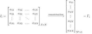
3. All images are N x N  matrices, which can be represented as N²  x 1 dimensional vectors. This is done by concatenating all the N rows of a matrix into a single row, which gives us a vector (a 1D array) of size N². The same logic would apply to images that are not of equal length and breadths. To take an example: An image of size 112 x 112 can be represented as a vector of dimension 12544 or simply as a point in a 12544 dimensional space.

Note: The face images need not be square matrices. We have considered images of dimension N x N, we could easily consider images of dimension m x N.

If you consider images of dimensions  m x N  then the vectorwould be of dimension  Nm x 1. The matrix A would then be of dimension mN x M, however AA^T or the covariance matrix C would always be a square matrix, irrespective of whether you choose square images or not.

The matrix  C would have to be a square matrix as we are interested in finding the eigenvectors, and eigenvectors are defined only for square matrices. I hope I could clear your doubt.

Algorithm for Finding Eigenfaces:

1. Obtain M training images  I₁, I₂, … I_{M ,} it is very important that the images are centered.

2. Represent each image I_i as a vectoras discussed above. This is done by concatenating all the rows of a matrix to form a vector, as shown below:

For illustration purposes, we can imagine the above operation to be taking place somewhat as shown below:

3. Find the average face vector

Average face (or mean face) obtained by finding

the average of all the face vectors in the data set

4. Subtract the mean face from each face vectorto get a set of vectors . The purpose of subtracting the mean image from each image vector is to be left with only the distinguishing features from each face and “removing”, in a way, information that is common.

Let A be a matrix containing the vectors Φ_i  column wise. i.e. 

5. Find the Covariance matrix C :

C = AA^T , where

Note that the Covariance matrix has simply been made by putting one modified image vector Φ_i in one column each. Also note that C is a N²  x N² matrix and A is a N²  x M matrix.

6. We now need to calculate the Eigenvectorsof  C . However note that C  is a N²  x N² matrix and it would return N² Eigenvectors each being N²dimensional. For an image this number is HUGE.  The computations required would easily make your system run out of memory. How do we get around this problem?

7. Instead of the Matrix AA^T consider the matrix A^TA. Remember A  is a N²  x M matrix, thus A^TA is a M x M  matrix. If we find the Eigenvectors of this matrix, it would return M Eigenvectors, each of dimension M x 1, let’s call these Eigenvectors.

Now from some properties of matrices, it follows that:. We have found outearlier. This implies that usingwe can calculate the M largest Eigenvectors of AA^T. Remember that M << N²  as M is simply the number of training images.

8. Find the best M Eigenvectors of  C = AA^T by using the relation discussed above. That is:. Also keep in mind that.

The M eigenvectors for the above set of M images will look something like as shown below:

9. Select the best K  Eigenvectors, the selection of these Eigenvectors is done heuristically.

[Best 6 Eigenfaces, assuming K=6]

Finding Weights:

The Eigenvectors found at the end of the previous section,when converted to a matrix in a process that is reverse to that in STEP 2, have a face like appearance. Since these are Eigenvectors and have a face like appearance, they are called Eigenfaces. Sometimes, they are also called as Ghost Images because of their weird appearance.

Now each face in the training set (minus the mean), Φ_i can be represented as a linear combination of these Eigenvectors :

,  where are Eigenfaces.

These weights can be calculated as :

Each normalized training image is represented in this basis as a vector.

where i = 1,2… M. This means we have to calculate such a vector corresponding to every image in the training set and store them as templates.

Recognition Task:

Now consider we have found out the Eigenfaces for the training images, their associated weights after selecting a set of most relevant Eigenfaces and have stored these vectors corresponding to each training image.

Given an unknown face image to recognize,

• Compute a "distance" between the new face and each of the training faces
• Select the training image that's closest to the new one as the most likely known person
• If the distance to that face image is above a threshold, "recognize" the image as that person, otherwise, classify the face as an "unknown" person

Deciding on the Threshold:

Why is the threshold important?

Consider for simplicity we have ONLY 5 images in the training set. And a probe that is not in the training set comes up for the recognition task. The score for each of the 5 images will be found out with the incoming probe. And even if an image of the probe is not in the database, it will still say the probe is recognized as the training image with which its score is the lowest. Clearly this is an anomaly that we need to look at. It is for this purpose that we decide the threshold. The threshold   is decided heuristically.

Now to illustrate what we just said, consider a simpson image as a non-face image, this image will be scored with each of the training images. Let’s say   is the lowest score out of all. But the probe image is clearly not belonging to the database. To choose the threshold we choose a large set of random images (both face and non-face), we then calculate the scores for images of people in the database and also for this random set and set the threshold    accordingly.

More on the Face Space:

Here is a brief discussion on the face space.

Consider a simplified representation of the face space as shown in the figure above. The images of a face, and in particular the faces in the training set should lie near the face space, which in general describes images that are face like.

The projection distance   should be under a threshold   as already seen. The images of known individual fall near some face class in the face space.

There are four possible combinations on where an input image can lie:

1. Near a face class and near the face space: This is the case when the probe is nothing but the facial image of a known individual (known = image of this person is already in the database).

2. Near face space but away from face class: This is the case when the probe image is of a person (i.e a facial image), but does not belong to anybody in the database i.e. away from any face class.

3. Distant from face space and near face class: This happens when the probe image is not of a face however it still resembles a particular face class stored in the database.

4. Distant from both the face space and face class: When the probe is not a face image i.e. is away from the face space and is nothing like any face class stored.

Out of the four, type 3 is responsible for most false positives. To avoid them, face detection is recommended to be a part of such a system.

Average-Half-Face

Several previous attempts to utilize the symmetry of the face for face recognition and face detection have been made. It is well-known that the “face is roughly symmetrical”. Zhao and Chellappa use the idea of face symmetry to solve the problem of illumination in face recognition using Symmetric Shape-from-Shading, while Ramanathan et al. introduce the notion of ‘Half-faces’ (in the sense of exactly one half of the face) to assist in computing a similarity measure between faces using images that have non-uniform illumination. In face recognition, the use of the bilateral symmetry of the face has been limited to extracting facial profiles for recognition.

The average-half-face is inspired by the symmetry preserving singular value decomposition (SPSVD). The SPSVD is used to reduce the dimensionality of data while simultaneously preserving symmetry that is present in the data. Singular Value Decomposition is a technique used in conjunction with Principal Component Analysis (PCA) during extraction of Eigenvectors. When applied to face images, this amounts to two steps. First, the image is centered about the nose of the (properly oriented) face to represent the data as symmetric as possible. When we speak of the data being symmetric, we mean that two spatial halves of the data are similar, not that the matrix of the data itself is symmetric. Next, the image is divided into two symmetric halves and they are averaged together (reversing the columns of one of the halves first). Thereafter, we forward this average-half face to the face recognition algorithm.

The figure above displays the full face image, the left and right faces after centering, and the average-half-face of an example image.

The average-half-face can be seen as a preprocessing step to a face recognition algorithm. Feature selection as well as subspace computation can be performed on the set of average-half-faces just as is done on a set of full faces. Therefore, the average-half-face can be applied to any face recognition algorithm that uses full frontal faces as an input.

Algorithm Outline:

1. Center and orient the face in the image. This is done in our work by using the location of the tip of the nose.

2. Partition the image into two equal left and right halves, I_l and I_r.

3. Reverse of the ordering of (or mirror) the columns of one of the images (in this case the right image), producing I_r’.

4. Average the resulting mirror right half image (I_r’) with the left half image (I_l) to produce the average-half face.

The average-half-face is then used in place of the full face image for face recognition. The face recognition algorithm uses eigenfaces to form two subspaces from the full face and average-half-face. Then, the classification of test faces is done separately in these subspaces.

I hope this post helped you. You are welcome to comment or ask questions. Au revoir!

References

·   Josh Harguess and J. K. Aggarwal.  “A Case for the Average-Half-Face in 2D and 3D for Face Recognition”

·   "Eigenface." Wikipedia, The Free Encyclopedia.        http://en. wikipedia.org/wiki/Eigenface

·    “Eigenvector.” Wikipedia, The Free Encyclopedia.        http://en.wikipedia.org/wiki/Eigenvector

·    “Facial Recognition System.” Wikipedia, The Free Encyclopedia.  http://en.wikipedia.org/wiki/Facial_recognition_system

·    “Principal Component Analysis.” Wikipedia, The Free Encyclopedia.   http://en.wikipedia.org/wiki/Principal_component_analysis

·   “Eigenface Tutorial.” Drexel University. http://www.pages.drexel.edu/~sis26/Eigenface-Tutorial.htm

·   Shubhendu Trivedi. “Face Recognition using Eigenfaces and Distance Classifiers: A Tutorial”, February 11, 2009.         http://onionesquereality.wordpress.com/2009/02/11/

·   Face-Recognition-using-Eigenfaces-and-Distance-Classifiers-A-Tutorial-Onionesque-Reality.htm/

·    “Seeing With OpenCV, Part 4: Face Recognition With Eigenface.”  Cognotics http://www.cognotics.com/opencv/servo_2007_series/part_4/index.html

·   Shang-Hung Lin. “An Introduction to Face Recognition Technology”

·   Jonathon Shlens. “A Tutorial on Principal Component Analysis.”  Center for Neural Science, New York University

·   Tarun Bhatia. “Principal Component Analysis (Dimensionality Reduction)”

·   “Principal Component Analysis.”  Nonlinear Dynamics Inc.  http://www.nonlinear.com/products/progenesis/samespots/Principal-component-analysis/

·   Andrew Davison. “Face Recognition”.                http://fivedots.coe.psu.ac.th/~ad/jg

·   Josh Harguess and J. K. Aggarwal.  “Is There a Connection Between Face  Symmetry and Face Recognition?”